Set 2D Maple plot options
These 2D Maple plot options are:
- Used within the plot statement argument (plotstatement) of the plotmaple command.
- Entered as equations of the form of option=value after the function(s), horizontal range, and vertical range. Example — plotmaple("plot(sin(x), x=-Pi..Pi, filled=true, title=`My Plot`)");
IMPORTANT: You can only have 1 set of quotations in your plotmaple function.
Example — $a=plotmaple("plot(sin(x), x = -2*Pi .. 2*Pi, title = "Sine\nGraph", titlefont = ["Roman", 15])"); will give an error.
Example — $a=plotmaple("plot(sin(x), x = -2*Pi .. 2*Pi, title = `Sine\nGraph`, titlefont = [`Roman`, 15])"); will be displayed properly.
TIP: Check out Set 3D Maple plot options to create 3D Maple plots.
Available 2D Maple plot options
TIP: Check out MapleTM Online Help for more details on 2D Maple plot options.
| 2D Maple plot option | Default setting (if applicable) | Description |
|---|---|---|
| adaptive | true |
When plotting a function over an interval, the interval is sampled at a number of points, controlled by sample and numpoints. NOTE: With the default setting of true, intervals are subdivided—at most—6 times in trying to improve the plot. Adaptive plotting, where necessary, subdivides these intervals to attempt to get a better representation of the function. This sub-sampling can be turned off by setting the adaptive option to false. By setting this option to a non-negative integer, you can control the maximum number of times that sub-intervals are divided. |
| axes |
Specifies the type of axes. Choose from: boxed, frame, none, or normal. | |
| axesfont |
Font for the labels on the tick marks of the axes (specified in the same manner as font). Overrides values specified for font. | |
| axis |
Specifies information about the x -axis and y-axis. axis=t applies the information given in t to both axes. axis[dir]=t allows the information to be specified for a single axis, with dir taking the value 1 ( x -axis) or 2 ( y -axis). TIP: Check out MapleTM Online Help for more information on axis. | |
| axiscoordinates | Cartesian |
The coordinate system used for display of the axes. The value t can be either polar or Cartesian. If t is polar, then radial and angular axes are generated. This option is used together with coords=polar. NOTE: This option is only available in the Standard interface. In the Classic interface, the coordinates are always Cartesian. |
| caption | no caption |
The caption printed under the plot (rendered in the image), and the alt-text readable by a screen reader for accessibility purposes. The value c can be a list consisting of the caption text followed by the font option. TIP: Check out MapleTM Online Help for more information on caption. |
| captionfont |
Specifies the font for a plot caption (specified in the same manner as font). Overrides values specified for font. | |
| color |
Specifies the color of the curves to be plotted. n should be spelled without capital letters. Example — blue, not Blue. TIP: Check out MapleTM Online Help for more information on color. | |
| colorscheme |
Specifies a color scheme to a surface or set of points. t should be spelled without capital letters. Example — blue, not Blue. TIP: Check out MapleTM Online Help for more information on colorscheme. | |
| coordinateview |
This option is used only when the axiscoordinates=polar. When that's the case, then r1..r2 specifies the radial range that's to be displayed, and a1..a2 specifies the angular range. | |
| coords | Cartesian |
The coordinate system. The value cname is a choice from the list of coords. To generate polar axes with polar plots, use the axiscoordinates=polar option along with the coords=polar option. TIP: Check out MapleTM Online Help for more information on coords. |
| discont |
Allows detection of discontinuities. TIP: Check out MapleTM Online Help for more information on discont. | |
| filled |
If set to true, the area between the curve and the x-axis is given a solid color. The value of the filled option can also be a list containing 1 or more sub-options (color, style, or transparency). The options in the list are applied only to the filled area, and not to the original curve itself. NOTE: This option doesn't work with non-Cartesian coordinate systems. | |
| filledregions |
If set to true, the regions defined by the curves are filled with different colors. Only valid with the following commands: contourplot, implicitplot, and listcontplot. NOTE: This option doesn't work with non-Cartesian coordinate systems. | |
| font |
Defines the font for the plot title, caption, axis tickmark labels, and axis labels if no values have been specified for the axesfont, captionfont, labelfont, or titlefont options. The value l is a list of the form [family, style, size]. The value of family can be: Times, Courier, Helvetica, or Symbol. TIP: family can also be any font name supported by your system. Example — Tahoma and Lucida in Windows. NOTE: The first letter of the family value must be capitalized. style can be omitted or can be: roman, bold, italic, bolditalic, oblique, or boldoblique. NOTE: The Symbol family doesn't accept a style option. size is the point size to be used. | |
| gridlines | false |
When gridlines=true or gridlines is provided, default gridlines are drawn. For greater gridline control, use the axis option. If the axis option is also provided and contains a gridlines sub-option, then that option overrides this gridlines option. |
| labeldirections | horizontal |
Specifies the direction in which labels are printed along the axes. The values of x and y must be horizontal or vertical. |
| labelfont |
Font for the labels on the axes of the plot (specified in the same manner as font). Overrides values specified for font. | |
| labels | the names of the variables in the original function to be plotted (if available) |
Specifies labels for the axes. If labels aren't specified and there aren't available variable names in the plotted function, no labels are applied. TIP: Check out MapleTM Online Help for more information on labels. |
| legend |
Legend entry for a plot. If the plot function is being used to plot multiple curves, then s can be a list containing a legend entry for each curve. NOTE: A set can't be used as it doesn't preserve the order of the legend entries. TIP: Check out MapleTM Online Help for more information on legend. | |
| legendstyle |
Legend style for a plot (specified in the same manner as font).. The value s is a list consisting of 1 or more sub-options. The sub-options available for legendstyle include font=f and location=loc. The location=loc sub-option allows values for loc to be: top, bottom, right, or left. | |
| linestyle | solid |
Controls the line style of curves. t can be an integer from 1 to 7, where each integer represents a line style, as given in the order of: (1) solid, (2) dot, (3) dash, (4) dashdot, (5) longdash, (6) spacedash, or (7) spacedot. t can also be the name of an available line styles. Example — dash |
| numpoints | 200 |
Specifies the minimum number of points to be generated. NOTE: plot employs an adaptive plotting scheme which automatically does more work where the function values don't lie close to a straight line. Hence, plot often generates more than the minimum number of points. |
| resolution | 800 |
Sets the horizontal display resolution of the device in pixels. n is used to determine when the adaptive plotting scheme terminates. A higher value results in more function evaluations for non-smooth functions. NOTE: This option is applicable only when adaptive plotting is used. |
| sample |
A list of numerical values which is to be used for the initial sampling of the function. Normally, the function is sampled at additional points. To restrict sampling to only these values, include adaptive=false when calling the plot function. | |
| scaling | unconstrained (plot is scaled to fit the window) |
Specifies the scaling of the graph. The constrained value causes all axes to use the same scale. Example — A circle appears perfectly round. |
| size |
Specifies the size of the plot window. You can set the size of the plot window by specifying the number of pixels, a proportion of worksheet width, a ratio (Example — a square), the golden ratio, or a custom ratio. w (width) must be a positive numeric value or the string default. h (height) must be a positive numeric value, or: default, golden, or square. If w or h is a number greater than or equal to 10, it specifies the number of pixels for the width or height. If w or h is default, then the default size (which may be interface-specific) is used. If w is a number less than 10, then the plot window width is w multiplied by the width of the worksheet. NOTE: This form for w is ignored if the plot is part of a plot array. If h is a number less than 10, then the height is h multiplied by the width of the plot window as given by w. If h is square, then this is equivalent to h having the value 1.0. If h is golden, then this is equivalent to h having the value equal to the reciprocal of the golden ratio ( 1/2 + sqrt(5)/2 ). | |
| style | polygonoutline |
The plot style can be: line, point, pointline, polygon (or patchnogrid), or polygonoutline (or patch). line, polygon, and polygonoutline all draw curves by interpolating between the sample points. The point style results in a plot of the points only. NOTE: polygonoutline draws any polygons as filled with an outline. polygon shows the polygons with no outline, whereas line draws the polygons as outlines only. pointline is a combination of point and line. |
| symbol |
Specifies the symbol to use for plotted points. Choose from: asterisk, box, circle, cross, diagonalcross, diamond, point, solidbox, solidcircle, or soliddiamond. | |
| symbolsize | 10 |
The size (in points) of a symbol used in plotting can be given by a positive integer. NOTE: This doesn't affect symbol=point. |
| thickness | 1 |
Specifies the thickness of lines in the plot. n must be a non-negative number. A value of 0 produces the thinnest line that looks good in most contexts. |
| tickmarks |
m and n specify the tickmark placement for the x-axis and y-axis, respectively. Choose from: an integer specifying the number of tickmarks, a list of values specifying locations, a list of equations each having the form location=label, a name, or a spacing structure. For greater control over the appearance of tickmarks, use the axis option. If the axis option is also provided and contains a tickmarks sub-option, then that option overrides this tickmarks option. TIP: Check out MapleTM Online Help for more information on tickmarks. | |
| title | no title |
The title for the plot. t can be an arbitrary expression. t can also be a list consisting of the title followed by the font option. TIP: Check out MapleTM Online Help for more information on title. |
| titlefont |
Font for the title of the plot (specified in the same manner as font). Overrides values specified for font. | |
| transparency |
Specifies the transparency of the plot surface. t must evaluate to a floating-point number in the range 0 to 1. A value of 0 means opaque. A value of 1 means fully transparent. | |
| view |
Indicates the minimum and maximum coordinates of the curve to be displayed on the screen. NOTE: The plot structure is analyzed to determine a reasonable view that allows you to see the significant features of the data. The coordinateview option is normally used with polar plots. NOTE: If the same option is provided more than once, with different values, then the final value specified is generally what is used. NOTE: The options described above are all available for the Standard Worksheet interface. |
Examples of 2D Maple plots
Here are some examples of using 2D Maple plot options within the plotstatement argument:
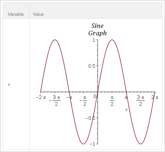
Example 1
Use the following 2D Maple plot options:
- title = `Sine\nGraph`
- titlefont = [`Roman`, 15]
Enter into the Algorithm Editor:
$a=plotmaple("plot(sin(x), x = -2*Pi .. 2*Pi, title = `Sine\nGraph`, titlefont = [`Roman`, 15])");
- Returns:
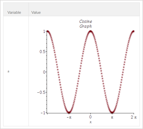
Example 2
Use the following 2D Maple plot options:
- title = `Cosine\nGraph`
- axes = framed
- style = point
- symbol = asterisk
- symbolsize = 15
- tickmarks = [spacing (Pi), default]
Enter into the Algorithm Editor:
$a=plotmaple("plot(cos(x), x = -2*Pi .. 2*Pi, title = `Cosine\nGraph`, axes = framed, style = point, symbol = asterisk, symbolsize = 15, tickmarks = [spacing(Pi), default])");
- Returns:
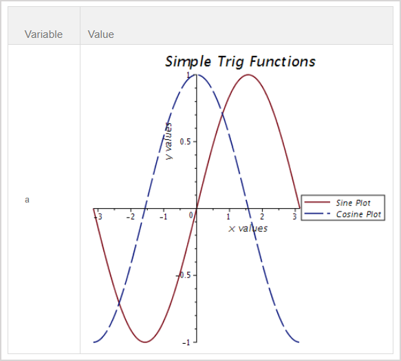
Example 3
Use the following 2D Maple plot options:
- title = `Simple Trig Functions`
- legend = [`Sine Plot`, `Cosine Plot`]
- titlefont = [`Roman`, 15]
- labels = [`x values`, `y values`]
- labeldirections = [`horizontal`, `vertical`]
- labelfont = [`Helvetica`, 10]
- linestyle = [solid, longdash]
- axesfont = [`Helvetica`, `Arial`, 8]
- legendstyle = [font = [`Helvetica`, 9], location = right])
Enter into the Algorithm Editor:
$a=plotmaple("plot([sin, cos], -Pi .. Pi, title = `Simple Trig Functions`, legend = [`Sine Plot`, `Cosine Plot`], titlefont = [`Arial`, 15], labels = [`x values`, `y values`], labeldirections = [`horizontal`, `vertical`], labelfont = [`Helvetica`, 10], linestyle = [solid, longdash], axesfont = [`Helvetica`, `Roman`, 8], legendstyle = [font = [`Helvetica`, 9], location = right])");
- Returns:
NOTE: titlefont, labelfont, and axesfont can be replaced by the font option as follows:
- font = [title, `Roman`, 15]
- font = [label, `Helvetica`, 10]
- font = [axes, `Helvetica`, `Roman`, 8]
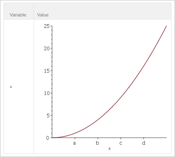
Example 4
Use the following 2D Maple plot options:
- tickmarks = [[1=`a`, 2=`b`, 3=`c`, 4=`d`], default])
Enter into the Algorithm Editor:
$a=plotmaple("plot(x^2, x = 0 .. 5, tickmarks = [[1 = `a`, 2 = `b`, 3 = `c`, 4 = `d`], default])");
- Returns:
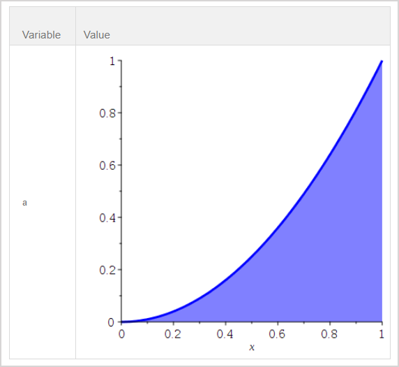
Example 5
Use the following 2D Maple plot options:
- color = `blue`
- thickness = 3
- filled = [color = `blue`, transparency = 0.5]
Enter into the Algorithm Editor:
$a=plotmaple("plot(x^2, x = 0 .. 1, color = `blue`, thickness = 3, filled = [color = `blue`, transparency = 0.5])");
- Returns: